Project 2: Fun with Filters and Frequencies!

Part 1: Fun with Filters

In this part, we build intuitions about 2D convolutions and filtering.
This is done primarily through visualizing what convolutions with the derivative look like.
IMPORTANT NOTE: For clarity, this webpage contains a link where images before and after alignment are displayed. For the webpage pdf, this other page has been attached at the bottom for convenience of viewing. Clicking links to Images and Cropped Images below will lead to the aforementioned pages.

Part 1.1: Finite Difference Operator

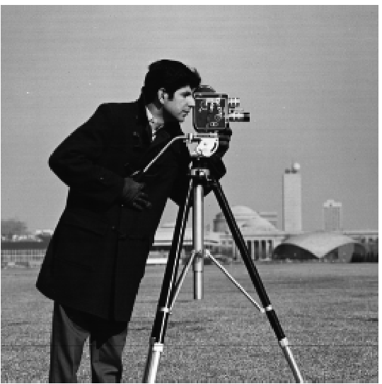
Our goal here is to visually see what the convolutions $f\star D_x$ and $f\star D_y $ do to an image $f$, where $D_x = \begin{bmatrix} 1 & -1 \end{bmatrix} $ and $ D_y = \begin{bmatrix} 1 \\ -1 \end{bmatrix} $ are finite difference operators. This is done with the cameraman image

cameraman.png

To see results, click on the following link:
Part 1.1 Results

Part 1.2: Derivative of Gaussian (DoG) filters

Our goal here is to experiment with Derivative of Gaussian filters, done again with the cameraman image.
To see results, click on the following link:
Part 1.2 Results

Part 2:

We will be able to create various interesting images (sharper images from blurred ones, hybrid images, blended images) using tricks with frequency and the Gaussian.

Part 2.1: Image Sharpening

Let $G$ be a Gaussian Filter and let $I$ be the identity filter. If $f\star G$ blurs an image, then for $\alpha > 0$ we can use the formula $ f - f\star G$ to construct an image of "details". Then \[ f_s(\alpha) = f + \alpha(f-f\star G) = f\star[ (1+\alpha) I - \alpha G ] \] is a sharpened image i.e. an image with more details.
To see results, click on the following link:
Part 2.1 Results

Part 2.2: Hybrid Images

We take as input images im1 and im2 , and wish to construct a combined image im that looks like im1 at high frequencies and im2 at low frequencies. This can be accomplished by taking Gaussian filters $ g_1 := g_1(\sigma_1,k) $ and $g_2 := g_2(\sigma_2,k) $ based on empirically chosen deviations and window size $ [6\sigma] + 1$, chosen to be sufficient to fit three standard deviations (most of the variation of a Gaussian) inside the Gaussian kernel. We generate low frequency im1 by convolution with Gaussian $ g_1$. We generate high frequency im2 via $\texttt{im2} \gets \texttt{im2} - \texttt{im2} \star g_2 $. Summing these images and normalizing, we have our desired hybrid image. From nearby, it should look like the high frequency image, and from further away it looks like the low frequency image.
To see results, click on the following link:
Part 2.2 Results

Part 2.3: Gaussian and Laplacian Stacks

A Gaussian Stack is a sequence of images where each subsequent image is given from the previous one via convolution with a Gaussian: \[ g_{i+1} = g_i \star \textup{Gauss}(\sigma_{i+1},k) \] where $ \sigma_{i+1} = 2\sigma_i $ and $ \sigma_0 $ is chosen. In a certain sense, they give blurrier and blurrier versions of the first image. A Laplacian stack is defined as having \[ \ell_{i+1} = g_{i+1} - g_i \], where $ g_i$ is the $i$th image in the Gaussian stack. It records the difference in details (or the details lost) between convolving by a certain $g_i$.
To see results, click on the following link:
Part 2.3 Results

Part 2.4: Multi-Resolution Blending

We use Masking in order to blend images together and create interesting visuals. The idea is to sum various layers of the Laplacian pyramid of an image with an appropriate mask filter applied to the two images being blended. To see results, click on the following link:
Part 2.4 Results